poems: Pattern-oriented ensemble modeling and simulation

The poems package provides a framework of interoperable R6 classes for building ensembles of viable models via the pattern-oriented modeling (POM) approach (Grimm et al., 2005). The package includes classes for encapsulating and generating model parameters, and managing the POM workflow. The workflow includes: model setup; generating model parameters via Latin hypercube sampling; running multiple sampled model simulations; collating summary results; and validating and selecting an ensemble of models that best match known patterns. By default, model validation and selection utilizes an approximate Bayesian computation (ABC) approach (Beaumont, Zhang, & Balding, 2002), although alternative user-defined functionality could be employed. The package also includes a spatially explicit demographic population model simulation engine, which includes default functionality for density dependence, correlated environmental stochasticity, stage-based transitions, and distance-based dispersal. The user may customize the simulator by defining functionality for translocations, harvesting, mortality, and other processes, as well as defining the sequence order for the simulator processes. The framework could also be adapted for use with other model simulators by utilizing its extendable (inheritable) base classes.

Framework and workflow

The poems framework utilizes a hierarchy of extendable (inheritable) R6 class objects that work together to manage a POM workflow for building an ensemble of simulation models.

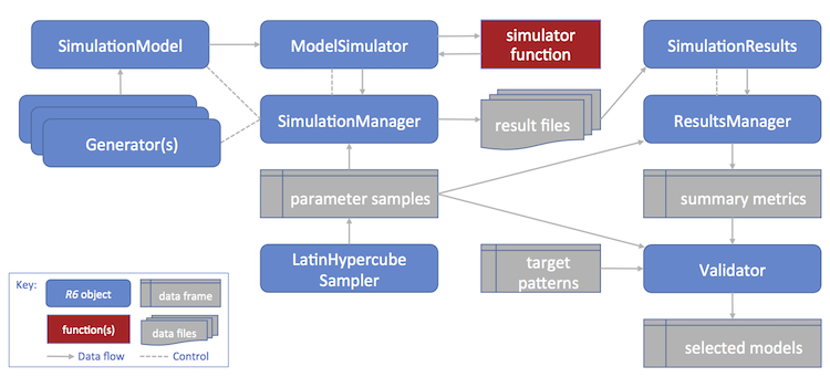
Create a simulation model template (a SimulationModel or inherited class object) with appropriate fixed parameters for the study domain. Also define a study region via the Region class if the simulations are to be spatially explicit.
Create generators (Generator or inherited class objects) for dynamically generating (non-singular) model parameters represented by data structures, such as arrays or lists.
Generate a data frame of sampled variable model parameters using the LatinHypercubeSampler. This will include singular model parameter values as well as input parameters for the generators.
Create a SimulationManager object configured with the simulation model (template), the generators, and the sample parameter data frame. Running this manager sets and runs the models via the simulator function for each set (row) of sampled parameters, utilising the generators when required. The results of each model simulation run are written to a file. A simulation log file is also created.
Create a ResultsManager object configured with the sample parameter data and result file details. Running this manager constructs a data frame of configured summary metrics, one row for each simulation result file. The manager utilizes the SimulationResults (or inherited) class to encapsulate, and dynamically generate additional derived, results. The metrics are generated via user-defined specifications and functions for calculating each metric from the results (objects).
Create a Validator object configured with the sample parameter data, summary metrics, and target (observed) pattern values for each metric. By default, the validator utilizes an approximate Bayesian computation (ABC) validation method via the abc library, although the validator (call) function can be configured to utilize other library or user-defined functions. Running the validator (with appropriate call function configuration) produces an ensemble of models (indices to sampled parameters) that were found to best match the targets. Diagnostic outputs may also be produced (depending on the call function and its configuration).
The selected models may then be utilized for further studies, such as alternative model scenarios or counterfactuals. This can be achieved by utilizing the selected subset of parameter samples to form inputs for further model simulations (by repeating the steps above).

Population modeling components

population_simulator function: The simulation engine's main function processes the model input parameters, controls the flow, calling other function modules as required, and returns the results of each simulation.
population_density function: Module for configuring and performing density dependence calculations at each simulation time step. A user-defined function may be utilized.
population_env_stoch function: Module for configuring and stochastically applying environmental variability to stage-based population transition rates at each simulation time step.
population_transitions function: Module for configuring and performing stage-based demographic transitions of population abundances at each simulation time step.
population_transformation function: Module for configuring and performing user-defined transformations to staged population abundances. This functionality is utilized when defining functions for translocation, harvest, mortality, or other custom transformative functions.
population_dispersal function: Module for configuring and performing dispersal calculations at each simulation time step. A user-defined function may be utilized.
population_results function: Module for configuring, initializing, and collating simulation results.
PopulationModel class: Inherited from SimulationModel, this class encapsulates the input parameters utilized by the population_simulator.
SimulatorReference class: This simple R6 class enables user-defined functionality to maintain persistent (attached) attributes and to write to the simulator results.
SpatialCorrelation class: Provides functionality for generating parameters that can be utilized when optionally applying a spatial correlation within the simulator's environmental variability calculations.
DispersalGenerator class: Inherited from Generator, this class provides functionality for generating distance-based dispersal parameters that can be utilized when performing dispersal calculations.
DispersalFriction class: Provides functionality for adjusting the (equivalent) distance between population cells given a spatio-temporal frictional landscape. These adjustments may be utilized by the DispersalGenerator.
PopulationResults class: Inherited from SimulationResults, this class encapsulates the results generated by the population_simulator, as well as dynamically generating additional derived results.

References

Beaumont, M. A., Zhang, W., & Balding, D. J. (2002). 'Approximate Bayesian computation in population genetics'. Genetics, vol. 162, no. 4, pp, 2025–2035.

Grimm, V., Revilla, E., Berger, U., Jeltsch, F., Mooij, W. M., Railsback, S. F., Thulke, H. H., Weiner, J., Wiegand, T., DeAngelis, D. L., (2005). 'Pattern-Oriented Modeling of Agent-Based Complex Systems: Lessons from Ecology'. Science vol. 310, no. 5750, pp. 987–991.

Examples

# Here we demonstrate building and running a simple population model. For a
# demonstration of the POM workflow with the model, see vignette("simple_example").

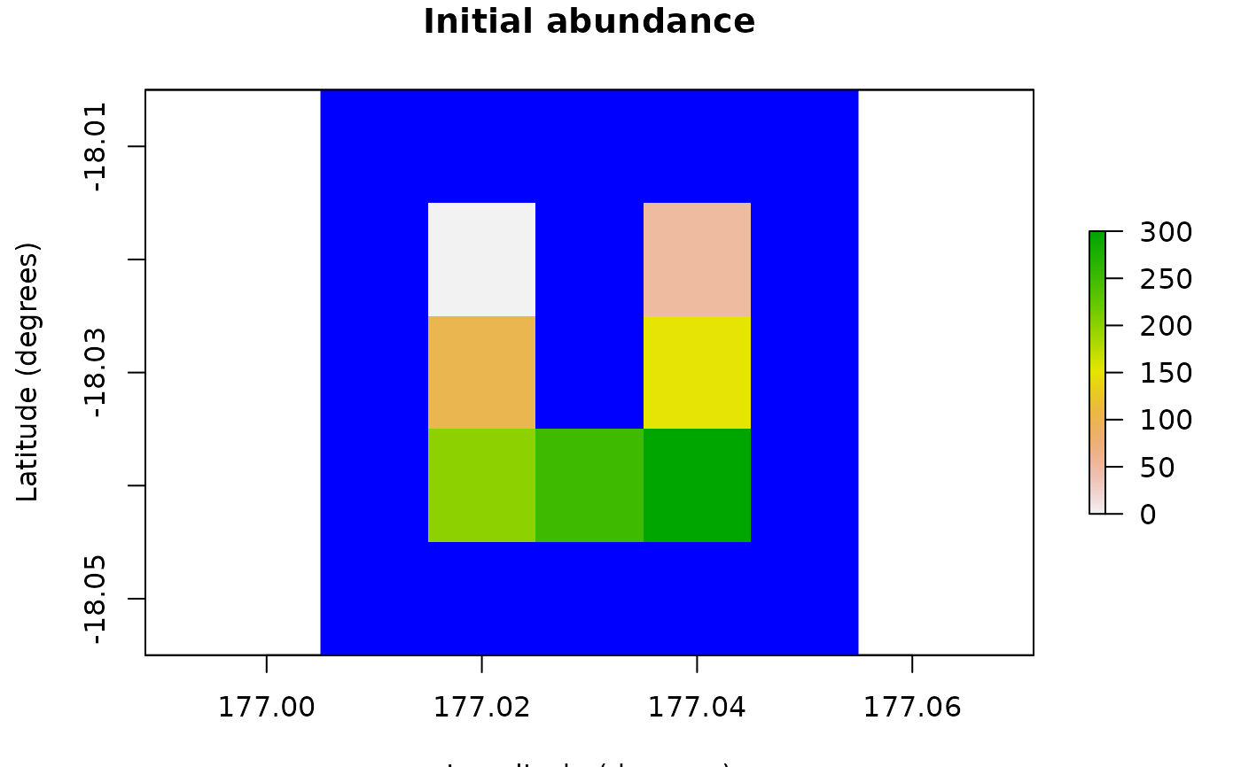
# Demonstration example region (U Island) and initial abundance
coordinates <- data.frame(
  x = rep(seq(177.01, 177.05, 0.01), 5),
  y = rep(seq(-18.01, -18.05, -0.01), each = 5)
)
template_raster <- Region$new(coordinates = coordinates)$region_raster # full extent
template_raster[][-c(7, 9, 12, 14, 17:19)] <- NA # make U Island
region <- Region$new(template_raster = template_raster)
initial_abundance <- seq(0, 300, 50)
raster::plot(region$raster_from_values(initial_abundance),
  main = "Initial abundance", xlab = "Longitude (degrees)",
  ylab = "Latitude (degrees)", zlim = c(0, 300), colNA = "blue"
)


# Set population model
pop_model <- PopulationModel$new(
  region = region,
  time_steps = 5,
  populations = 7,
  initial_abundance = initial_abundance,
  stage_matrix = matrix(c(
    0, 2.5, # Leslie/Lefkovitch matrix
    0.8, 0.5
  ), nrow = 2, ncol = 2, byrow = TRUE),
  carrying_capacity = rep(200, 7),
  density_dependence = "logistic",
  dispersal = (!diag(nrow = 7, ncol = 7)) * 0.05,
  result_stages = c(1, 2)
)

# Run single simulation
results <- population_simulator(pop_model)
results # examine
#> $all
#> $all$abundance
#> [1] 1032 1137 1264 1278 1301
#> 
#> $all$abundance_stages
#> $all$abundance_stages[[1]]
#> [1] 606 693 771 759 752
#> 
#> $all$abundance_stages[[2]]
#> [1] 426 444 493 519 549
#> 
#> 
#> 
#> $abundance
#>      [,1] [,2] [,3] [,4] [,5]
#> [1,]   50  115  153  185  187
#> [2,]   87  130  170  157  160
#> [3,]  133  163  192  177  173
#> [4,]  170  171  186  187  193
#> [5,]  194  175  180  181  206
#> [6,]  183  187  198  190  178
#> [7,]  215  196  185  201  204
#> 
#> $abundance_stages
#> $abundance_stages[[1]]
#>      [,1] [,2] [,3] [,4] [,5]
#> [1,]   31   65   95  109  114
#> [2,]   52   81  106   90   91
#> [3,]   77   98  129   99  115
#> [4,]  103  102  105  121  107
#> [5,]  119   97  112  105  117
#> [6,]  105  117  125  115   94
#> [7,]  119  133   99  120  114
#> 
#> $abundance_stages[[2]]
#>      [,1] [,2] [,3] [,4] [,5]
#> [1,]   19   50   58   76   73
#> [2,]   35   49   64   67   69
#> [3,]   56   65   63   78   58
#> [4,]   67   69   81   66   86
#> [5,]   75   78   68   76   89
#> [6,]   78   70   73   75   84
#> [7,]   96   63   86   81   90
#> 
#> 
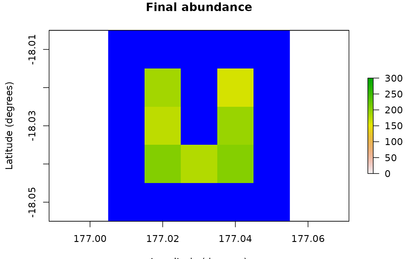
raster::plot(region$raster_from_values(results$abundance[, 5]),
  main = "Final abundance", xlab = "Longitude (degrees)",
  ylab = "Latitude (degrees)", zlim = c(0, 300), colNA = "blue"
)